Time series forecasting
Features that are extracted with tsfresh can be used for many different tasks, such as time series classification,
compression or forecasting.
This section explains how one can use the features for time series forecasting tasks.
The “sort” column of a DataFrame in the supported Data Formats gives a sequential state to the
individual measurements. In the case of time series this can be the time dimension while in the case of spectra the
order is given by the wavelength or frequency dimensions.
We can exploit this sequence to generate more input data out of a single time series, by rolling over the data.
Lets say you have the price of a certain stock, e.g. Apple, for 100 time steps.
Now, you want to build a feature-based model to forecast future prices of the Apple stock.
So you will have to extract features in every time step of the original time series while looking at
a certain number of past values.
A rolling mechanism will give you the sub time series of last m time steps to construct the features.
The following image illustrates the process:
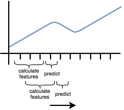
So, we move the window that extract the features and then predict the next time step (which was not used to extract features) forward.
In the above image, the window moves from left to right.
Another example can be found in streaming data, e.g. in Industry 4.0 applications.
Here you typically get one new data row at a time and use this to for example predict machine failures. To train your model,
you could act as if you would stream the data, by feeding your classifier the data after one time step,
the data after the first two time steps etc.
Both examples imply, that you extract the features not only on the full data set, but also
on all temporal coherent subsets of data, which is the process of rolling. In tsfresh, this is implemented in the
function tsfresh.utilities.dataframe_functions.roll_time_series().
Further, we provide the tsfresh.utilities.dataframe_functions.make_forecasting_frame() method as a convenient
wrapper to fast construct the container and target vector for a given sequence.
The rolling mechanism
The rolling mechanism takes a time series  with its data rows
 ![[x_1, x_2, x_3, ..., x_n]](../_images/math/908802a646a69f8414f225d4703cb20014d4297f.png) and creates
and creates  new time series
  , each of them with a different consecutive part
of :
, each of them with a different consecutive part
of :
To see what this does in real-world applications, we look into the following example flat DataFrame in tsfresh format
| id |
time |
x |
y |
|---|
| 1 |
t1 |
1 |
5 |
| 1 |
t2 |
2 |
6 |
| 1 |
t3 |
3 |
7 |
| 1 |
t4 |
4 |
8 |
| 2 |
t8 |
10 |
12 |
| 2 |
t9 |
11 |
13 |
where you have measured the values from two sensors x and y for two different entities (id 1 and 2) in 4 or 2 time
steps (t1 to t9).
Now, we can use tsfresh.utilities.dataframe_functions.roll_time_series() to get consecutive sub-time series.
E.g. if you set rolling to 0, the feature extraction works on the original time series without any rolling.
So it extracts 2 set of features,
| id |
time |
x |
y |
|---|
| 1 |
t1 |
1 |
5 |
| 1 |
t2 |
2 |
6 |
| 1 |
t3 |
3 |
7 |
| 1 |
t4 |
4 |
8 |
and
| id |
time |
x |
y |
|---|
| 2 |
t8 |
10 |
12 |
| 2 |
t9 |
11 |
13 |
If you set rolling to 1, the feature extraction works with all of the following time series:
| id |
time |
x |
y |
|---|
| 1 |
t1 |
1 |
5 |
| 1 |
t2 |
2 |
6 |
| id |
time |
x |
y |
|---|
| 1 |
t1 |
1 |
5 |
| 1 |
t2 |
2 |
6 |
| 1 |
t3 |
3 |
7 |
| 2 |
t8 |
10 |
12 |
| id |
time |
x |
y |
|---|
| 1 |
t1 |
1 |
5 |
| 1 |
t2 |
2 |
6 |
| 1 |
t3 |
3 |
7 |
| 1 |
t4 |
4 |
8 |
| 2 |
t8 |
10 |
12 |
| 2 |
t9 |
11 |
13 |
If you set rolling to -1, you end up with features for the time series, rolled in the other direction
| id |
time |
x |
y |
|---|
| 1 |
t3 |
3 |
7 |
| 1 |
t4 |
4 |
8 |
| id |
time |
x |
y |
|---|
| 1 |
t2 |
2 |
6 |
| 1 |
t3 |
3 |
7 |
| 1 |
t4 |
4 |
8 |
| 2 |
t9 |
11 |
13 |
| id |
time |
x |
y |
|---|
| 1 |
t1 |
1 |
5 |
| 1 |
t2 |
2 |
6 |
| 1 |
t3 |
3 |
7 |
| 1 |
t4 |
4 |
8 |
| 2 |
t8 |
10 |
12 |
| 2 |
t9 |
11 |
13 |
We only gave an example for the flat DataFrame format, but rolling actually works on all 3 Data Formats
that are supported by tsfresh.
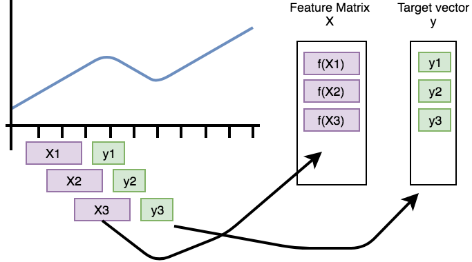
This process is also visualized by the following figure.
It shows how the purple, rolled sub-timeseries are used as base for the construction of the feature matrix X
(after calculation of the features by f).
The green data points need to be predicted by the model and are used as rows in the target vector y.
Parameters and Implementation Notes
The above example demonstrates the overall rolling mechanism, which creates new time series.
Now we discuss the naming convention for such new time series:
For identifying every subsequence, tsfresh uses the time stamp of the point that will be predicted as new “id”.
The above example with rolling set to 1 yields the following sub-time series:
| id |
time |
x |
y |
|---|
| t2 |
t1 |
1 |
5 |
| t2 |
t2 |
2 |
6 |
| id |
time |
x |
y |
|---|
| t3 |
t1 |
1 |
5 |
| t3 |
t2 |
2 |
6 |
| t3 |
t3 |
3 |
7 |
| id |
time |
x |
y |
|---|
| t4 |
t1 |
1 |
5 |
| t4 |
t2 |
2 |
6 |
| t4 |
t3 |
3 |
7 |
| t4 |
t4 |
4 |
8 |
| id |
time |
x |
y |
|---|
| t9 |
t8 |
10 |
12 |
| t9 |
t9 |
11 |
13 |
The new id is the time stamp where the shift ended.
So above, every table represents a sub-time series.
The higher the shift value, the more steps the time series was moved into the specified direction (into the past in
this example).
If you want to limit how far the time series shall be shifted into the specified direction, you can set the
max_timeshift parameter to the maximum time steps to be shifted.
In our example, setting max_timeshift to 1 yields the following result (setting it to 0 will create all possible shifts):
| id |
time |
x |
y |
|---|
| t2 |
t1 |
1 |
5 |
| t2 |
t2 |
2 |
6 |
| id |
time |
x |
y |
|---|
| t3 |
t2 |
2 |
6 |
| t3 |
t3 |
3 |
7 |
| id |
time |
x |
y |
|---|
| t4 |
t3 |
3 |
7 |
| t4 |
t4 |
4 |
8 |
| id |
time |
x |
y |
|---|
| t9 |
t8 |
10 |
12 |
| t9 |
t9 |
11 |
13 |
![\hat x^k = [x_k, x_{k-1}, x_{k-2}, ..., x_1]](../_images/math/929828003d21836b7ed01e8ecd150780de4fc9e5.png)